

Risk And Return
/How to Improve Your Portfolio's Sharpe Ratio
How to Improve Your Portfolio's Sharpe Ratio
Follow one recognizable portfolio through a full workflow — review its baseline, clone it, improve its diversification, optimize the weights, and compare the result with the original.
A portfolio's Sharpe Ratio improves in one of two ways: earn more return without adding proportional volatility, or reduce volatility while preserving return. The most reliable lever is not finding a single high-Sharpe asset — it is changing how your holdings combine and what weight each one carries.
This guide works through that process on a single, well-known portfolio. We start on the published page for the classic four-asset Permanent Portfolio, use its indicators as the baseline, then clone it and use PortfoliosLab's diversification and optimization tools to raise its Sharpe Ratio. You can follow the same steps on a portfolio you already own.
For what the Sharpe Ratio measures and when it can mislead, see Sharpe Ratio Explained.
Asset Sharpe Is Not Portfolio Sharpe
A fund with a strong standalone Sharpe Ratio does not automatically improve your portfolio. A lower-Sharpe fund can add more value when its returns behave differently from your existing holdings. The test that matters is whether the fund improves the combined portfolio's return relative to its total volatility.
The Workflow
1
Open and clone the starting portfolio
Review the published portfolio’s Sharpe Ratio, return, volatility, and drawdown, then clone it to create an editable working copy.
2
Check diversification
Use portfolio clusters to see whether four holdings really provide four independent sources of behavior.
3
Rebuild the bond sleeve
Preserve the 50% bond allocation while replacing SHY and TLT with two funds selected by trading history and low correlation, then compare the result with the original.
4
Optimize the weights
Run Mean-Variance Optimization with a Minimize Drawdown objective, a 7% target return, and a walk-forward backtest to improve the diversified portfolio further.
5
Compare with the original
Judge the proposed portfolio against the baseline on Sharpe, return, volatility, drawdown, and concentration — not Sharpe alone.
The Sample Portfolio
The Permanent Portfolio, popularized by Harry Browne, splits capital equally across four assets meant to each do well in a different economic environment:
| Symbol | Holding | Weight |
|---|---|---|
| VTI | Vanguard Total Stock Market ETF | 25% |
| TLT | iShares 20+ Year Treasury Bond ETF | 25% |
| SHY | iShares 1-3 Year Treasury Bond ETF | 25% |
| GLD | SPDR Gold Shares | 25% |
It is a good teaching case because the four sleeves are genuinely different, so diversification analysis has something real to show. But the equal 25% split is a rule of thumb, not a Sharpe-optimal allocation — the short-term Treasury sleeve drags return while the long-bond sleeve carries outsized volatility. That leaves clear room to improve risk-adjusted performance without abandoning the portfolio's logic.
Step 1 — Open and Clone the Portfolio
Open the Permanent Portfolio and review the indicators on its portfolio page. These published results provide the baseline for every later step, so you do not need to recreate the portfolio in Portfolio Analysis first.
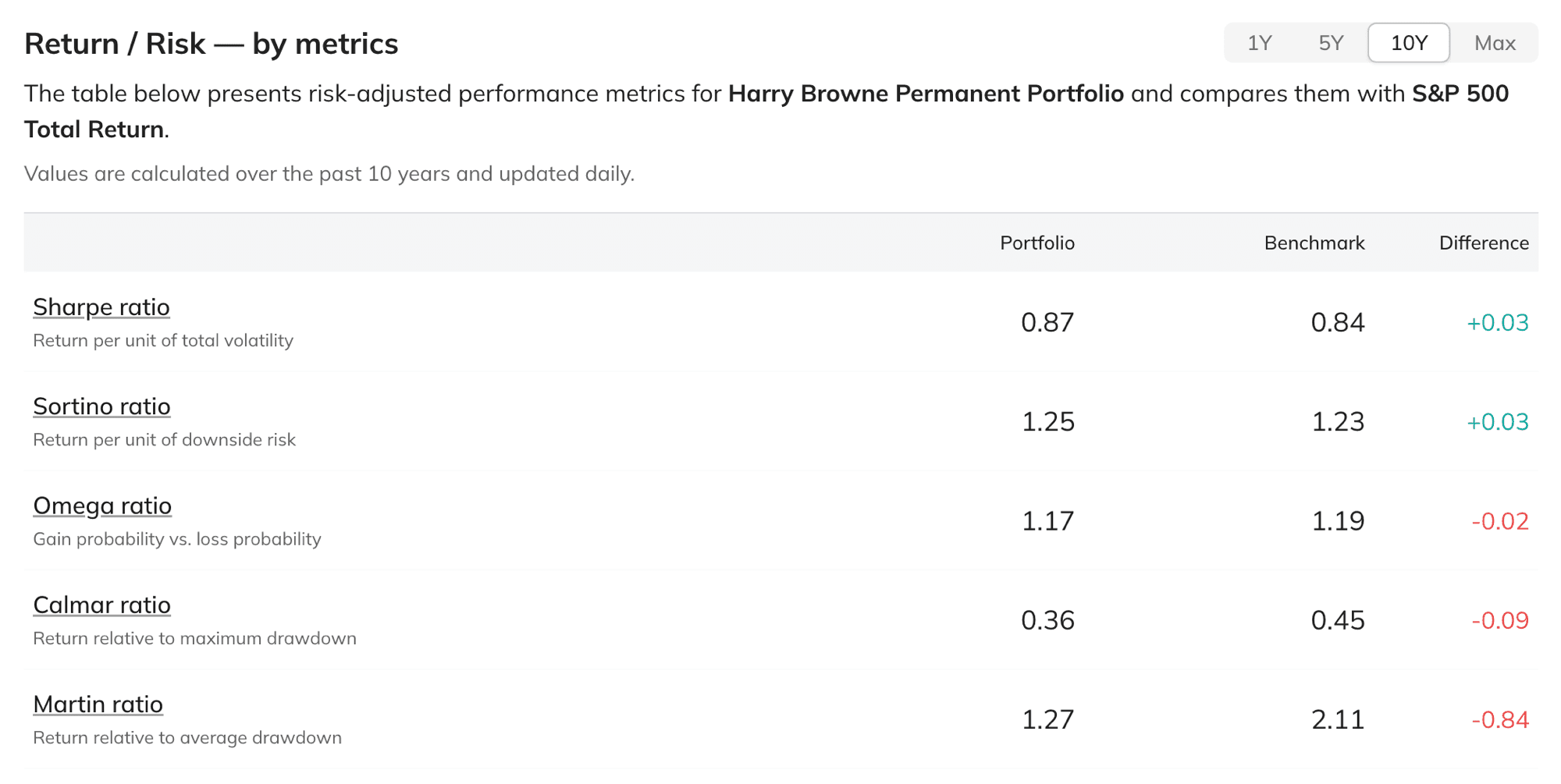
For a more stable baseline, use the trailing 10-year figures shown on the page as of July 17, 2026:
- Sharpe Ratio: 0.87
- Annualized return: 6.76%
- Volatility: 7.77%
- Maximum drawdown: -18.99%
After recording the baseline, click Clone the portfolio on the same page and save the copy to your account. The clone gives you an editable portfolio to load into the tools used in the remaining steps while the published portfolio stays available as the original reference.
The Portfolio Analysis guide explains the result sections in more detail. Note the Sharpe Ratio in particular — improving it is the goal of every step that follows.
Step 2 — Check Diversification
Open Diversification Analysis, load the cloned portfolio, and review the correlation matrix and clusters together. The point is to see where the portfolio's risk and return actually come from before changing anything.
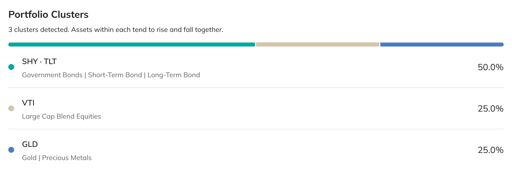
The analysis detects three clusters rather than four. SHY and TLT form a single government-bond cluster and together account for 50% of the portfolio, while VTI and GLD each form a distinct 25% cluster. Stocks, gold, and government bonds provide three different return drivers, but half of the allocation remains concentrated in one broad bond group.
This does not make SHY or TLT redundant: short- and long-term Treasuries carry very different duration risk. It does create a clear target for the next step — preserve the portfolio's 50% bond sleeve while splitting it across two funds that do not fall into the same behavioral cluster.
The Understanding Diversification guide covers correlations, concentration, and the diversification ratio in more depth.
Step 3 — Rebuild the Bond Sleeve
The original portfolio has four tickers but behaves like a portfolio with three clusters. A simple response is to preserve its broad allocation — 25% stocks, 25% gold, and 50% bonds — while replacing the two funds inside the bond sleeve. This changes the diversification within fixed income without redesigning the entire strategy.
Start in the Portfolio Diversifiers section of Diversification Analysis and select the first candidate with at least ten years of trading history. In this snapshot, the first qualifying ticker is FLTR. Next, open FLTR Diversifiers and take the first fixed-income fund among the lowest-correlation results that also has at least ten years of history. That produces ULST.
This rule deliberately takes the first eligible fund at each stage instead of searching for the ETF with the best past return. That reduces hindsight bias and makes the method repeatable. Diversifier rankings change as prices and trading histories evolve, so the qualifying tickers you see may differ; follow the selection rule rather than forcing the same symbols.
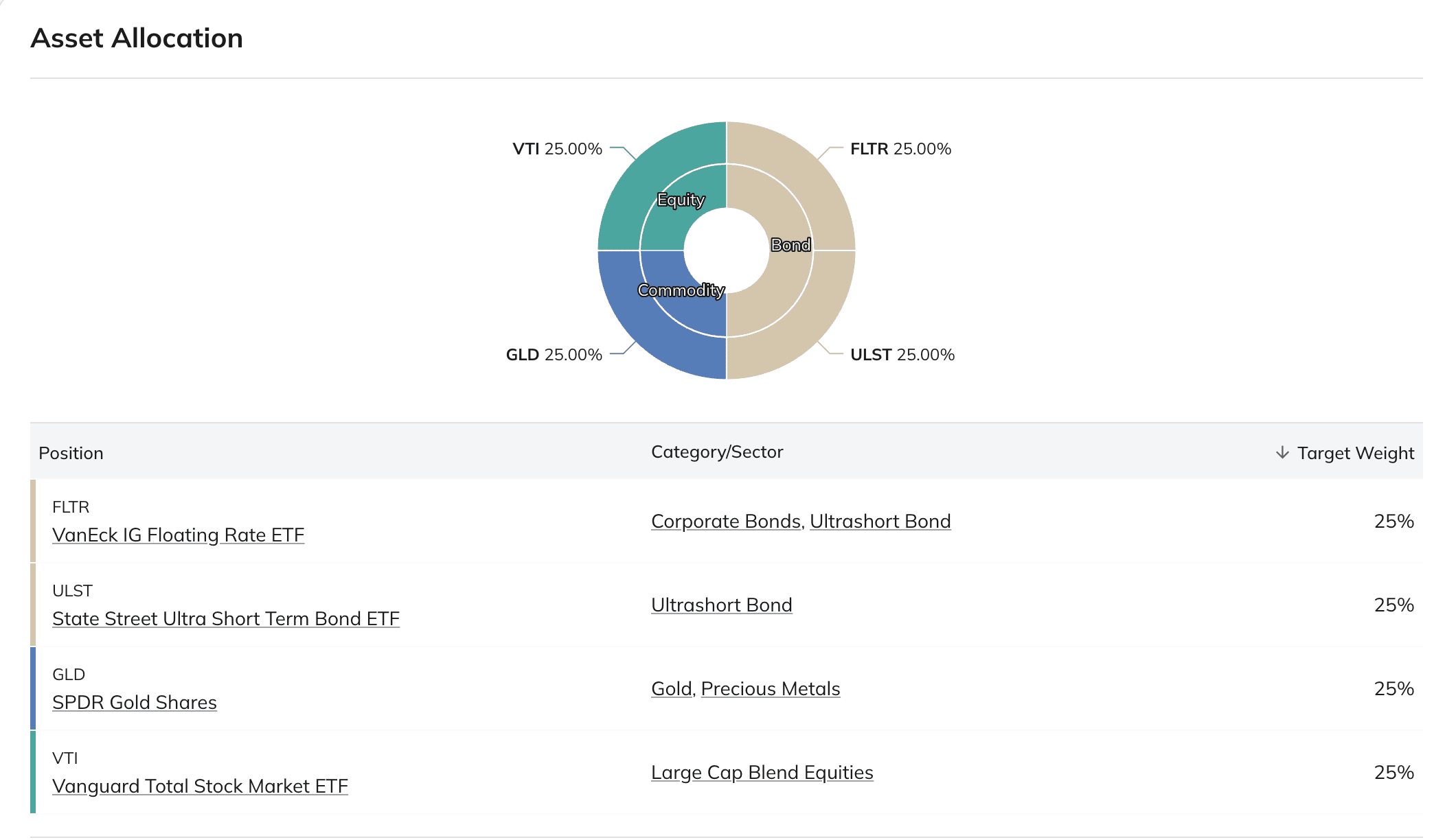
Replace SHY and TLT in the cloned portfolio with FLTR and ULST, leaving all four positions at 25%:
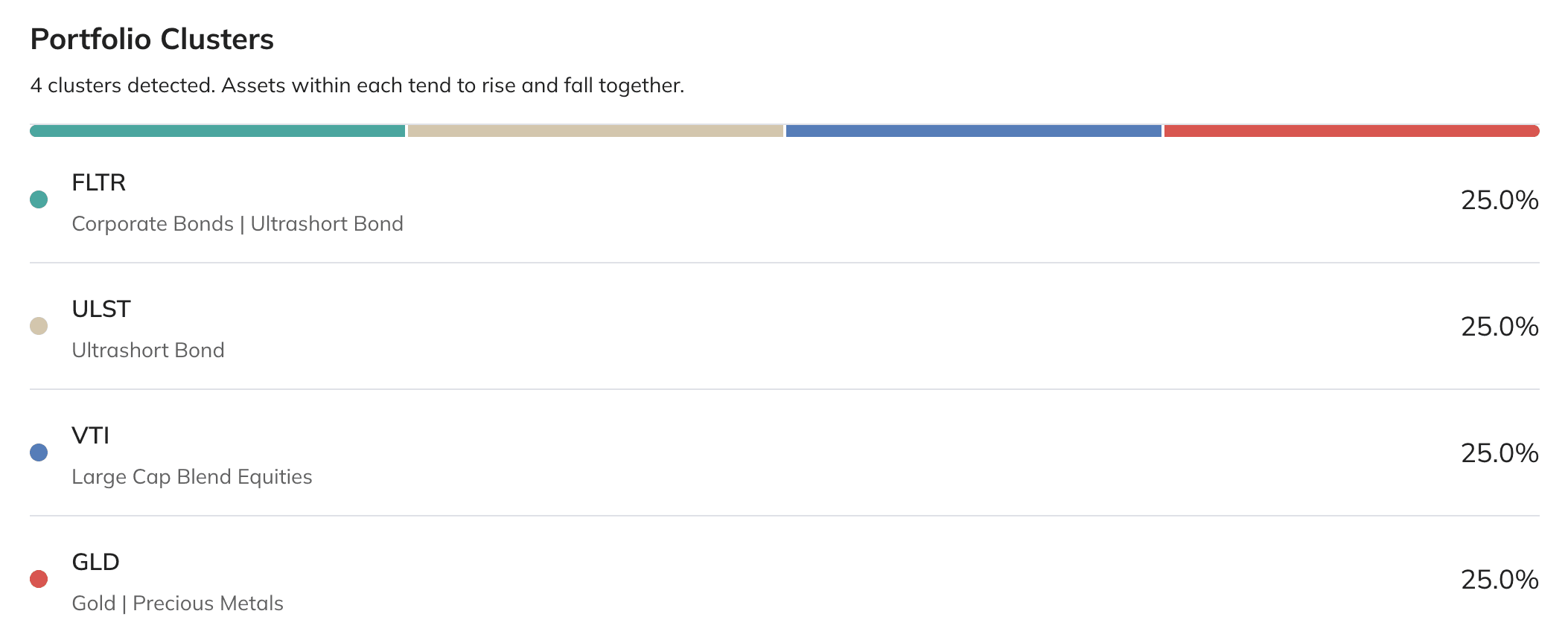
Run Diversification Analysis again before moving on. The revised portfolio now produces four clusters, one for each holding, instead of grouping the two bond funds together:
The asset correlation table confirms the separation. Pairwise correlations range from 0.01 to 0.20, and the correlation between FLTR and ULST is 0.08:
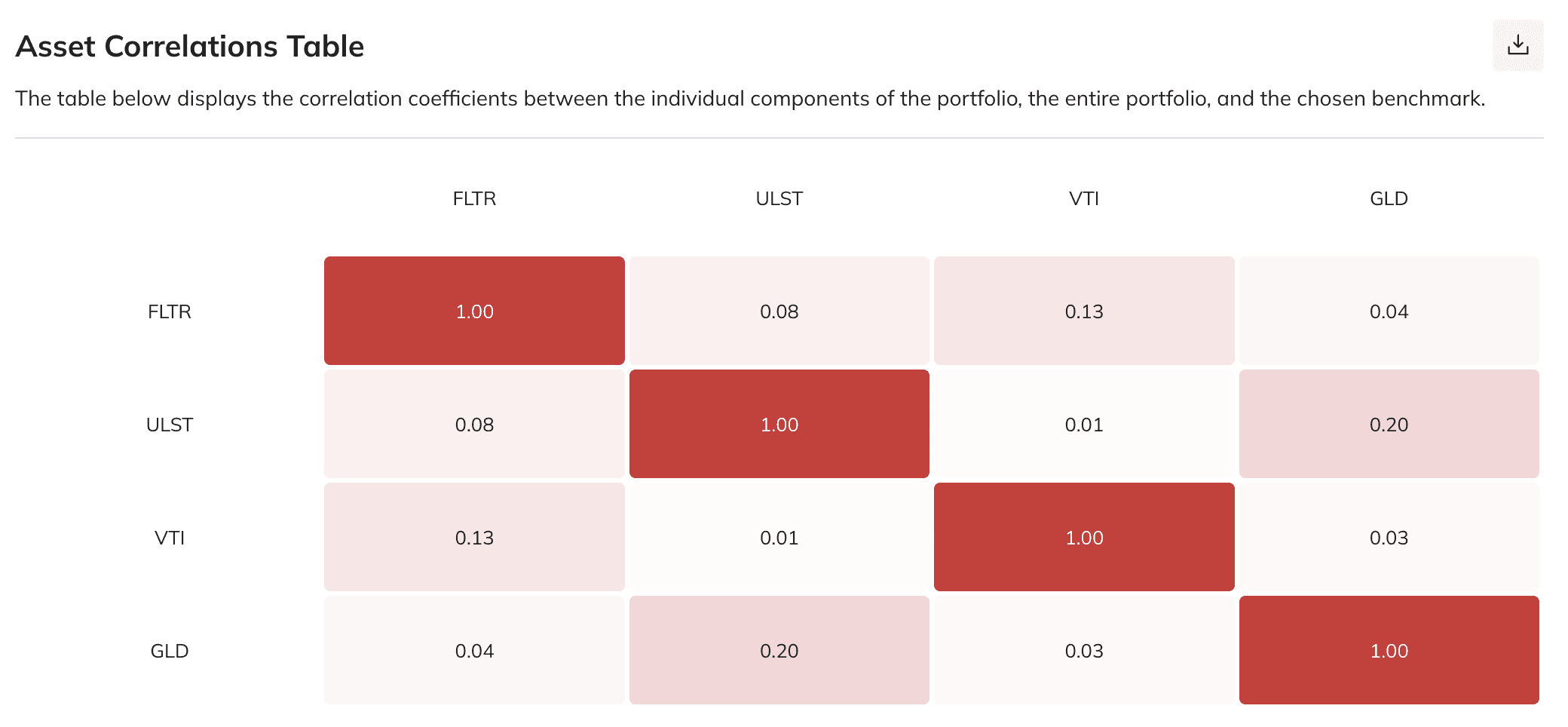
Four separate clusters show that the replacement changed how the holdings interact, but cluster separation alone does not prove that the portfolio's Sharpe Ratio improved. Save the revised portfolio as Permanent Diversified, open Portfolio Analysis, and select the original Permanent Portfolio as its benchmark.
The trailing 10-year performance chart already shows an improvement before any optimization. The diversified portfolio gains 125.66% versus 92.37% for the original, and its equity curve appears smoother with fewer pronounced pullbacks:
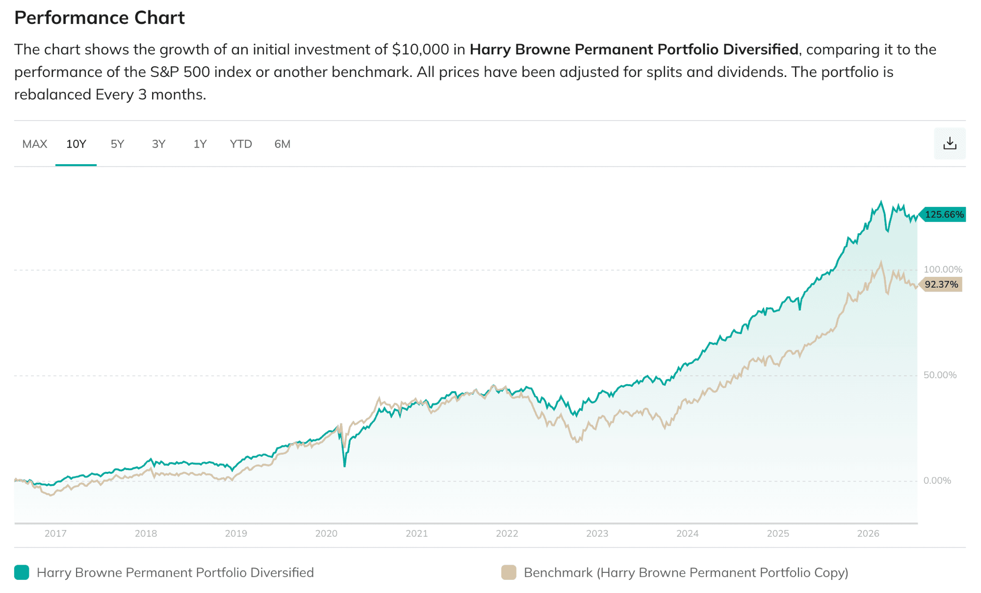
This is diversification in action: changing how the bond holdings behave improves the combined return path without selecting funds for their past returns. The 10-year risk-adjusted metrics confirm the gain. Sharpe rises from 0.87 to 1.23, Sortino from 1.25 to 1.67, Omega from 1.17 to 1.26, Calmar from 0.36 to 0.56, and Martin from 1.27 to 3.49:
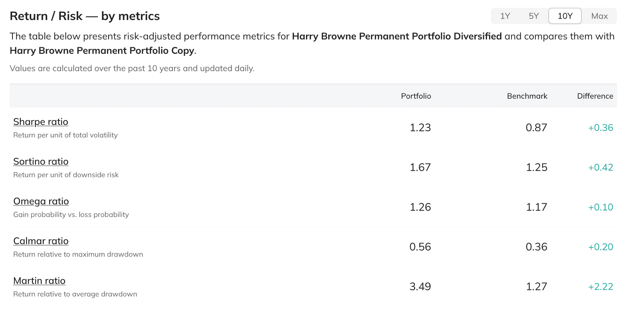
The portfolio has therefore improved through diversification alone. The next step checks whether optimizing the weights can extract additional risk-adjusted performance from the same four holdings.
Step 4 — Optimize the Weights
Open Portfolio Optimization and load Permanent Diversified. The bond replacement has already improved the equal-weight portfolio; this step tests whether a different allocation can improve it further.
Choose Mean-Variance Optimization with the Minimize Drawdown objective. Maximize Sharpe is also a valid objective, but minimizing drawdown provides more control over the return target. A 7% target annualized return approximately matches the original portfolio's 6.76% trailing 10-year return, allowing the optimizer to focus on reducing drawdowns without requiring a higher return.
Use these settings:
- Select Minimize Drawdown as the objective.
- Set the target annualized return to 7%.
- Choose a walk-forward backtest with quarterly optimization.
- Use a three-year training window.
- Set the minimum position weight to 10% so the optimizer cannot reduce a holding to a negligible allocation.
The walk-forward test simulates running the strategy consistently through time. At the start of each quarter, the optimizer uses only the preceding three years of returns to calculate the allocation, then holds those weights through the next quarter. The process repeats across the backtest, so every allocation is evaluated on data the optimizer did not see during training. This does not eliminate overfitting, but it is more realistic than fitting and evaluating the strategy on the same full historical period.
Unlike a one-time optimization, this walk-forward strategy does not have one static set of optimized weights. It starts with the VTI, FLTR, ULST, and GLD universe, recalculates the allocation every quarter from the latest three-year window, and keeps every position at or above 10%.
In the latest run, the optimizer allocates 70% to ULST and 10% each to FLTR, GLD, and VTI:
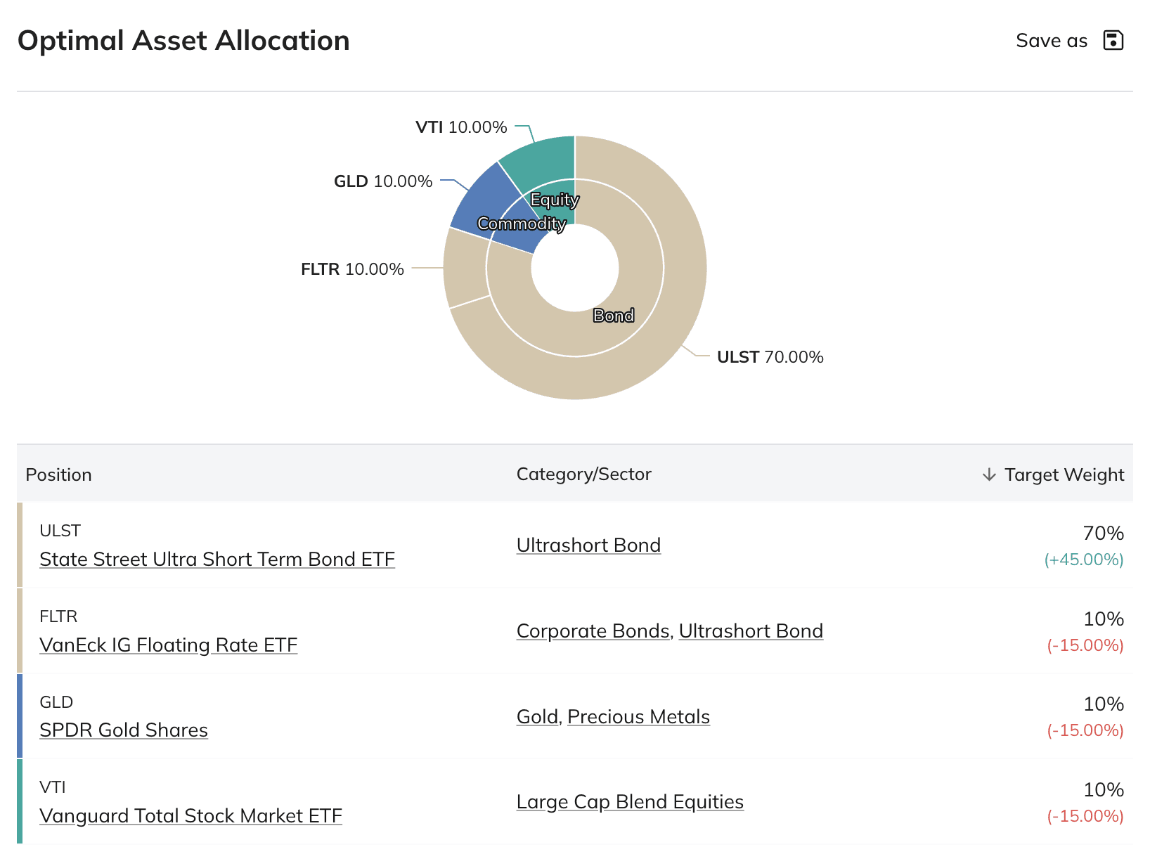
The 10% minimum prevents the optimizer from eliminating a holding, but it does not limit how large another position can become. Without a maximum-weight constraint, the latest allocation can still concentrate 70% in one fund.
The allocation-over-time chart shows the weights produced by every quarterly run. The mix changes substantially as each new three-year training window moves through different market conditions:
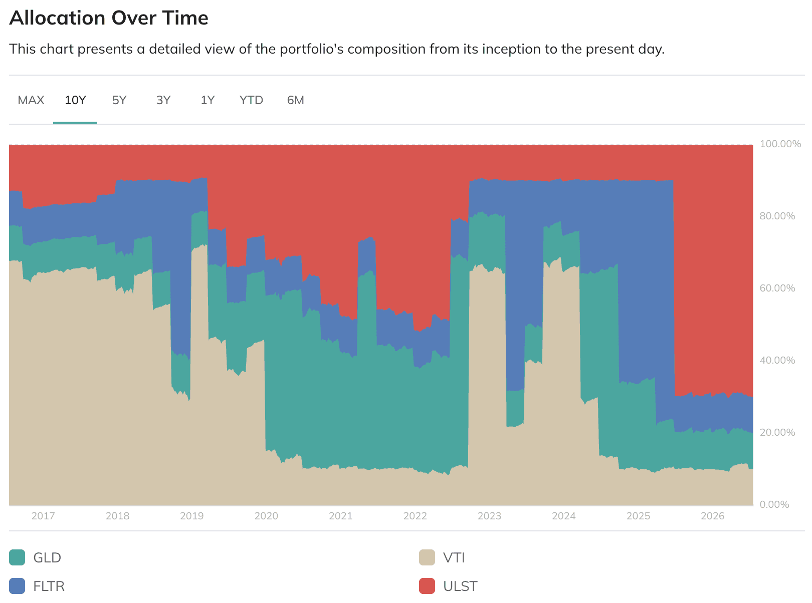
These changing weights — not the latest 70/10/10/10 snapshot applied retroactively — produce the walk-forward performance compared in the next step.
For the full settings reference, see Mean-Variance Optimization.
Step 5 — Compare With the Original
A higher backtested Sharpe is only meaningful next to the portfolios that came before it. The final performance chart contains all three stages: Optimized Portfolio is the walk-forward strategy, Original Portfolio is the equal-weight Permanent Diversified portfolio, and the benchmark is the original Harry Browne Permanent Portfolio.
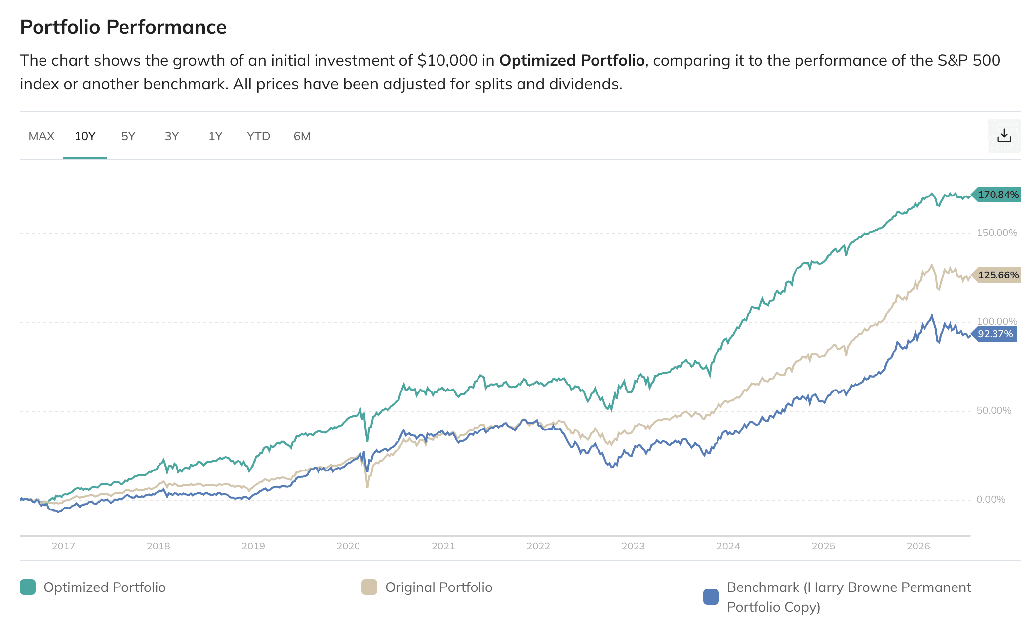
Over the trailing 10 years, the optimized strategy gains 170.84%, compared with 125.66% for the equal-weight diversified portfolio and 92.37% for the original Permanent Portfolio. The optimized curve also finishes with a shallower major drawdown than either comparison portfolio.
The period comparison shows how the optimization behaves across different market windows rather than presenting only the strongest result:
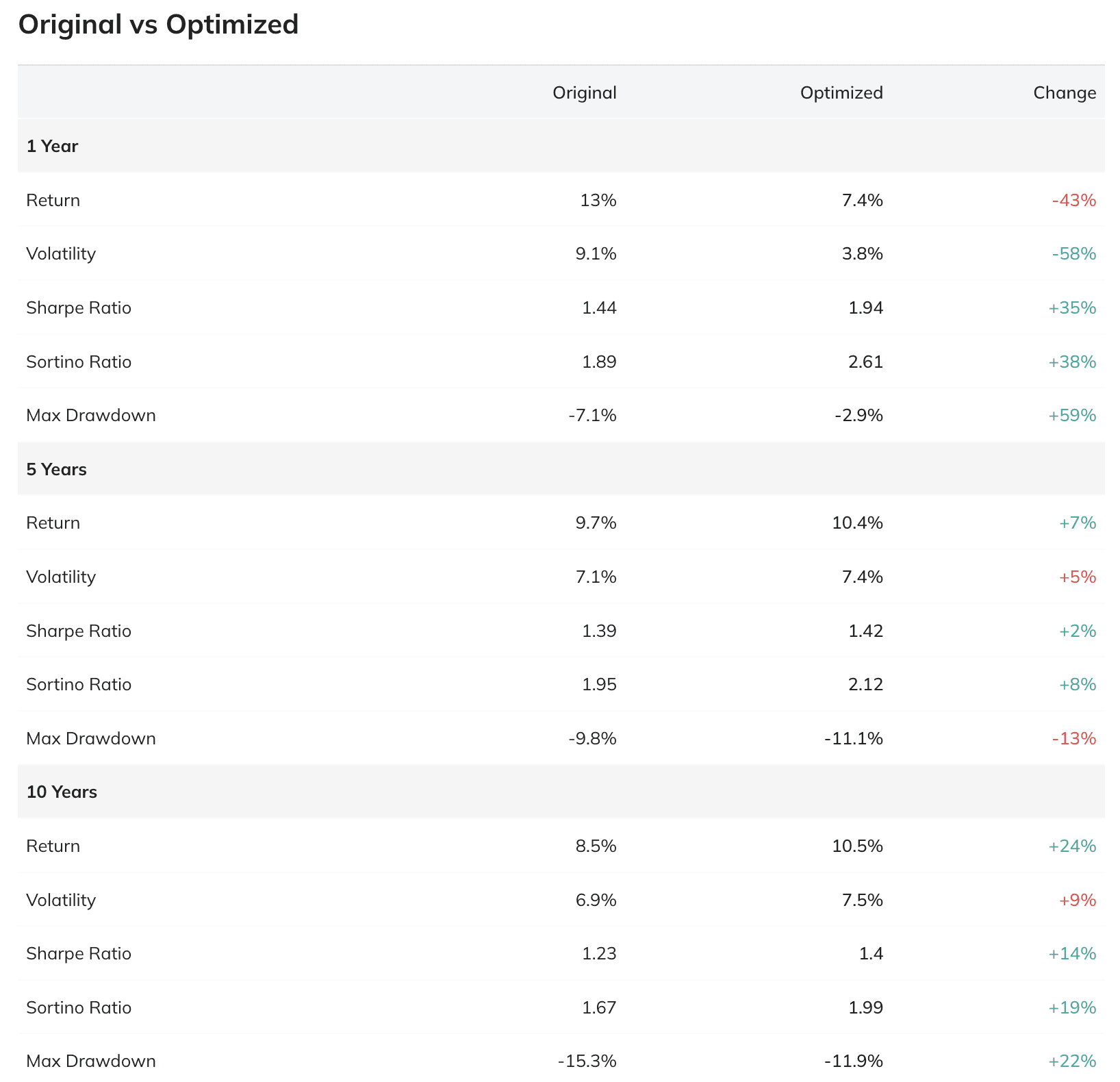
The trailing 10-year figures show the full progression. PortfoliosLab metrics update daily, so the exact values may shift over time:
| Metric | Original Permanent | Permanent Diversified | Optimized |
|---|---|---|---|
| Sharpe Ratio | 0.87 | 1.23 | 1.40 |
| Annualized return | 6.76% | 8.50% | 10.50% |
| Volatility | 7.77% | 6.90% | 7.50% |
| Maximum drawdown | -18.99% | -15.30% | -11.90% |
Over 10 years, optimization raises annualized return from 8.50% to 10.50%, Sharpe from 1.23 to 1.40, and Sortino from 1.67 to 1.99 while reducing maximum drawdown from -15.30% to -11.90%. Volatility rises from 6.90% to 7.50%, so the higher Sharpe comes from stronger returns and shallower drawdowns rather than lower volatility alone.
The optimizer is not better on every horizon. Its one-year return is lower than the equal-weight portfolio's, and its five-year volatility and maximum drawdown are slightly worse. Those tradeoffs are why the final decision should consider multiple periods and metrics instead of selecting the allocation from its 10-year Sharpe alone.
Guardrails
- Walk-forward testing avoids training on future observations, but results still depend on the chosen training window, optimization frequency, target return, and constraints.
- A 7% historical target does not guarantee that the portfolio will earn 7% in the future.
- A minimum-weight constraint keeps every holding in the portfolio but does not cap concentration. Add a maximum weight if a 70% allocation to one fund exceeds your risk tolerance.
- A high standalone Sharpe Ratio is a screening signal, not proof that an investment will improve the combined portfolio.
- The optimizer only works with the assets you supply. It can reweight a poorly diversified list, but it cannot add a missing asset class unless you do.
- Do not pick a fund on rank alone. Fees, drawdowns, category exposure, liquidity, and overlap with current holdings still matter. Validate the result with Maximum Drawdown, not Sharpe alone.
Conclusion
Two changes raised this portfolio's Sharpe Ratio from 0.87 to 1.40 without abandoning its four-asset logic: rebuilding the bond sleeve so the holdings stopped moving together, then letting the optimizer set the weights against a drawdown-aware objective. Neither step depended on finding a winning fund — both came from changing how the pieces combine, measured before and after on the same 10-year window.
The same sequence — establish a baseline, find where risk actually concentrates, diversify, optimize, then compare across periods — applies to any portfolio you already own. Run it on your own holdings and let the numbers, rather than instinct, show whether a change is a real improvement.
The funds and settings shown were chosen to demonstrate the workflow, not as recommendations. Do your own research on what fits your strategy.